Near to Far Field Spectra#
The near-to-far field transformation feature is demonstrated using four different examples. There are three steps involved in this type of calculation. First, the "near" surface(s) is defined as a set of surfaces capturing all outgoing radiation in the desired direction(s). Second, the simulation is run using a pulsed source (or alternatively, a CW source via the frequency-domain solver) to allow Meep to accumulate the DFT fields on the near surface(s). Third, Meep computes the far fields at any desired points with the option to save the far fields to an HDF5 file.
Radiation Pattern of an Antenna#
In this example, we compute the radiation pattern of an antenna. This involves an electric-current point dipole emitter in vacuum. The source is placed at the center of a 2d cell surrounded by PML. The near fields are obtained on a bounding box defined along the edges of the non-PML region. The far fields are computed in two ways from closed surfaces: (1) sides of a square and (2) circumference of a circle, having a length/radius many times larger than the source wavelength and lying beyond the cell. From both the near and far fields, we will also compute the total outgoing Poynting flux and demonstrate that they are equivalent. Results will be shown for three orthogonal polarizations of the input source.
The simulation geometry is shown in the following schematic.

In the first part of the simulation, we define the cell and source as well as the near field and flux regions. Since we are using a pulsed source (with center wavelength of 1 μm), the fields are timestepped until they have sufficiently decayed away.
The simulation script is in examples/antenna-radiation.ctl.
(set-param! resolution 50)   ; pixels/μm

(define-param sxy 4)
(define-param dpml 1)
(set! geometry-lattice (make lattice (size (+ sxy (* 2 dpml)) (+ sxy (* 2 dpml)) no-size)))

(set! pml-layers (list (make pml (thickness dpml))))

(define-param fcen 1.0)
(define-param df 0.4)
(define-param src-cmpt Ez)
(set! sources (list (make source
                      (src (make gaussian-src (frequency fcen) (fwidth df)))
                      (center 0)
                      (component src-cmpt))))

(if (= src-cmpt Ex)
    (set! symmetries (list (make mirror-sym (direction X) (phase -1))
                           (make mirror-sym (direction Y) (phase +1)))))
(if (= src-cmpt Ey)
    (set! symmetries (list (make mirror-sym (direction X) (phase +1))
                           (make mirror-sym (direction Y) (phase -1)))))
(if (= src-cmpt Ez)
    (set! symmetries (list (make mirror-sym (direction X) (phase +1))
                           (make mirror-sym (direction Y) (phase +1)))))

(define nearfield-box
  (add-near2far fcen 0 1
        (make near2far-region (center 0 (* +0.5 sxy)) (size sxy 0) (weight +1))
        (make near2far-region (center 0 (* -0.5 sxy)) (size sxy 0) (weight -1))
        (make near2far-region (center (* +0.5 sxy) 0) (size 0 sxy) (weight +1))
        (make near2far-region (center (* -0.5 sxy) 0) (size 0 sxy) (weight -1))))

(define flux-box
  (add-flux fcen 0 1
        (make flux-region (center 0 (* +0.5 sxy)) (size sxy 0) (weight +1))
        (make flux-region (center 0 (* -0.5 sxy)) (size sxy 0) (weight -1))
        (make flux-region (center (* +0.5 sxy) 0) (size 0 sxy) (weight +1))
        (make flux-region (center (* -0.5 sxy) 0) (size 0 sxy) (weight -1))))

(run-sources+ (stop-when-fields-decayed 50 src-cmpt (vector3 0 0) 1e-8))
After the time stepping, the flux of the near fields is computed using get-fluxes and displayed:
(print "near-flux:, " (list-ref (get-fluxes flux-box) 0) "\n")
In the first of two cases, the flux of the far fields is computed using the flux routine for a square box of side length 2 mm which is 2000 times larger than the source wavelength. This requires computing the outgoing flux on each of the four sides of the box separately and summing the values. The resolution of the far fields is chosen arbitrarily as 1 point/μm. This means there are 2x10⁶ points per side length.
(define-param r (/ 1000 fcen)) ; half side length of far-field square box OR radius of far-field circle
(define-param res-ff 1)        ; resolution of far fields (points/μm)
(define far-flux (+ (list-ref (flux nearfield-box Y (volume (center 0 r 0) (size (* 2 r) 0 0)) res-ff) 0)
                    (- (list-ref (flux nearfield-box Y (volume (center 0 (- r) 0) (size (* 2 r) 0 0)) res-ff) 0))
                    (list-ref (flux nearfield-box X (volume (center r 0 0) (size 0 (* 2 r) 0)) res-ff) 0)
                    (- (list-ref (flux nearfield-box X (volume (center (- r) 0 0) (size 0 (* 2 r) 0)) res-ff) 0))))

(print "far-flux-box:, " far-flux "\n")
For the second of two cases, we use the get-farfield routine to compute the far fields by looping over a set of 100 equally-spaced points along the circumference of a circle with radius of 1 mm. The six far field components (E, E, E, H, H, H) are displayed in separate columns as complex numbers.
(define-param npts 100)           ; number of points in [0,2*pi) range of angles
(map (lambda (n)
       (let ((ff (get-farfield nearfield-box (vector3 (* r (cos (* 2 pi (/ n npts)))) (* r (sin (* 2 pi (/ n npts)))) 0))))
     (print "farfield:, " n ", " (* 2 pi (/ n npts)))
     (map (lambda (m)
        (print ", " (list-ref ff m)))
          (arith-sequence 0 1 6))
     (print "\n")))
         (arith-sequence 0 1 npts))
The script is run and the output piped to a file using the following shell commands. The far field data is extracted from the output and placed in a separate file.
meep src-cmpt=Ez antenna-radiation.ctl |tee source_Jz_farfields.out
grep farfield: source_Jz_farfields.out |cut -d , -f2- > source_Jz_farfields.dat
From the far fields at each point , we compute using Matlab/Octave the outgoing or radial flux: , where P and P are the components of the Poynting vector . Note that is always 0 since this is a 2d simulation. The total flux is then computed and displayed:
d = dlmread("source_Jz_farfields.dat",",");

Ex = conj(d(:,3));
Ey = conj(d(:,4));
Ez = conj(d(:,5));

Hx = d(:,6);
Hy = d(:,7);
Hz = d(:,8);

Px = real(Ey.*Hz-Ez.*Hy);
Py = real(Ez.*Hx-Ex.*Hz);
Pr = sqrt(Px.^2+Py.^2);

r = 1000;    % radius of far-field circle
disp(sprintf("far-flux-circle:, %0.6f",sum(Pr)*2*pi*r/length(Pr)));
By Poynting's theorem, the total outgoing flux obtained by integrating around a closed surface should be the same whether it is calculated from the near or far fields (unless there are sources or absorbers in between). The flux of the near fields for the J source is 2.456196 and that for the far fields is 2.458030 (box) and 2.457249 (circle). The ratio of near- to far-field (circle) flux is 0.999571. Similarly, for the J source, the values are 1.227786 (near-field), 1.227651 (far-field box), and 1.227260 (far-field circle). The ratio of near- to far-field (circle) flux is 1.000429. The slight differences in the flux values are due to discretization effects and will decrease as the resolution is increased.
Finally, we plot the radial flux normalized by its maximum value over the entire interval to obtain a range of values between 0 and 1. These are shown below in the linearly-scaled, polar-coordinate plots. The three figures are obtained using separate runs involving a src-cmpt of E, E, and E. As expected, the J and J sources produce dipole radiation patterns while J has a monopole pattern.
angles = d(:,2);
polar(angles,Pr/max(Pr),'b-');
set(gca, 'xtick', [0 0.5 1.0]);

Focusing Properties of a Metasurface Lens#
This example demonstrates how to compute the far-field profile at the focal length of a metasurface lens. The lens design, which is also part of the tutorial, is based on a supercell of binary-grating unit cells. For a review of the binary-grating geometry as well as a demonstration of computing its phasemap, see Tutorial/Mode Decomposition/Phase Map of a Subwavelength Binary Grating. The far-field calculation of the lens contains two separate components: (1) compute the phasemap of the unit cell as a function of a single geometric parameter, the duty cycle, while keeping its height and periodicity fixed (1.8 and 0.3 μm), and (2) form the supercell lens by tuning the local phase of each of a variable number of unit cells according to the quadratic formula for planar wavefront focusing. The design wavelength is 0.5 μm and the focal length is 0.2 mm. The input source is an Ez-polarized planewave at normal incidence.
There are two simulation scripts: examples/metasurface_lens_phasemap.ctl and examples/metasurface_lens_farfield.ctl.
The first script takes three geometric input arguments (periodicity, height, and duty cycle) for a unit cell and computes the phase as well as the transmittance of the zeroth order. The phase value is then later translated from the range of [-π,π] of Mode Decomposition to [-2π,0] in order to be consistent with the analytic formula for the local phase. The second script computes the far-field intensity profile for a metasurface lens (a supercell formed from a list of duty cycles) around its focal length.
(set-param! resolution 50)  ; pixels/μm

(define-param dpml 1.0)     ; PML thickness
(define-param dsub 2.0)     ; substrate thickness
(define-param dpad 2.0)     ; padding between grating and PML
(define-param gp 0.3)       ; grating period
(define-param gh 1.8)       ; grating height
(define-param gdc 0.5)      ; grating duty cycle

(define sx (+ dpml dsub gh dpad dpml))
(define sy gp)

(define cell (make lattice (size sx sy no-size)))
(set! geometry-lattice cell)

(define boundary-layers (list (make pml (thickness dpml) (direction X))))
(set! pml-layers boundary-layers)

(define-param lcen 0.5)      ; center wavelength
(define fcen (/ lcen))       ; center frequency
(define df (* 0.2 fcen))     ; frequency width

(define pulse-src (list (make source
                          (src (make gaussian-src (frequency fcen) (fwidth df)))
                          (component Ez)
                          (center (+ (* -0.5 sx) dpml (* 0.5 dsub)) 0 0)
                          (size 0 sy 0))))

(set! sources pulse-src)

(set! k-point (vector3 0 0 0))

(define glass (make medium (index 1.5)))
(set! default-material glass)

(define symm (list (make mirror-sym (direction Y))))
(set! symmetries symm)

(define mon-pt (vector3 (- (* 0.5 sx) dpml (* 0.5 dpad)) 0 0))
(define flux-obj (add-flux fcen 0 1 (make flux-region (center mon-pt) (size 0 sy 0))))

(run-sources+ 50)

(define input-flux (get-fluxes flux-obj))

(reset-meep)

(set! geometry-lattice cell)

(set! pml-layers boundary-layers)

(set! sources pulse-src)

(set! k-point (vector3 0 0 0))

(set! default-material air)

(set! geometry (list (make block
                       (material glass)
                       (size (+ dpml dsub) infinity infinity)
                       (center (+ (* -0.5 sx) (* 0.5 (+ dpml dsub))) 0 0))
                     (make block
                       (material glass)
                       (size gh (* gdc gp) infinity)
                       (center (+ (* -0.5 sx) dpml dsub (* 0.5 gh)) 0 0))))

(set! symmetries symm)

(set! flux-obj (add-flux fcen 0 1 (make flux-region (center mon-pt) (size 0 sy 0))))

(run-sources+ 200)

(define res (get-eigenmode-coefficients flux-obj (list 1) #:eig-parity (+ ODD-Z EVEN-Y)))
(define coeffs (list-ref res 0))

(define mode-tran (/ (sqr (magnitude (array-ref coeffs 0 0 0))) (list-ref input-flux 0)))
(define mode-phase (angle (array-ref coeffs 0 0 0)))
(if (> mode-phase 0) (set! mode-phase (- mode-phase (* 2 pi))))

(print "mode:, " mode-tran ", " mode-phase "\n")
(set-param! resolution 50)  ; pixels/μm

(define-param dpml 1.0)     ; PML thickness
(define-param dsub 2.0)     ; substrate thickness
(define-param dpad 2.0)     ; padding between grating and PML
(define-param gp 0.3)       ; grating period
(define-param gh 1.8)       ; grating height

(define-param focal-length 200) ; focal length of metalens
(define-param spot-length 100)  ; far field line length
(define-param ff-res 10)        ; far field resolution (points/μm)

; list of grating duty cycles
(define-param gdc-list (list '()))

; # of cells
(define num-cells (length gdc-list))

; return gdc of nth cell
(define gdc-cell (lambda (n) (list-ref gdc-list n)))

(define sx (+ dpml dsub gh dpad dpml))
(define sy (* num-cells gp))

(define cell (make lattice (size sx sy no-size)))
(set! geometry-lattice cell)

(define boundary-layers (list (make pml (thickness dpml) (direction X))))
(set! pml-layers boundary-layers)

(define-param lcen 0.5)      ; center wavelength
(define fcen (/ lcen))       ; center frequency
(define df (* 0.2 fcen))     ; frequency width

(define pulse-src (list (make source
                          (src (make gaussian-src (frequency fcen) (fwidth df)))
                          (component Ez)
                          (center (+ (* -0.5 sx) dpml (* 0.5 dsub)) 0 0)
                          (size 0 sy 0))))

(set! sources pulse-src)

(set! k-point (vector3 0 0 0))

(define glass (make medium (index 1.5)))

(set! geometry (list (make block
                       (material glass)
                       (size (+ dpml dsub) infinity infinity)
                       (center (+ (* -0.5 sx) (* 0.5 (+ dpml dsub))) 0 0))))

(set! geometry (append geometry
                       (map (lambda (n)
                              (make block
                                (material glass)
                                (size gh (* (gdc-cell n) gp) infinity)
                                (center (+ (* -0.5 sx) dpml dsub (* 0.5 gh)) (+ (* -0.5 sy) (* (+ n 0.5) gp)) 0)))
                            (arith-sequence 0 1 num-cells))))

(define symm (list (make mirror-sym (direction Y))))
(set! symmetries symm)

(define mon-pt (vector3 (- (* 0.5 sx) dpml (* 0.5 dpad)) 0 0))
(define n2f-obj (add-near2far fcen 0 1 (make near2far-region (center mon-pt) (size 0 sy 0))))

(run-sources+ 500)

(output-farfields n2f-obj (string-append "numcells-" (number->string num-cells)) (volume (center (+ (* -0.5 sx) dpml dsub gh focal-length) 0 0) (size spot-length 0 0)) ff-res)
Using Octave/Matlab, in the first of two parts of the calculation, a phasemap of the binary-grating unit cell is generated based on varying the duty cycle from 0.1 to 0.9.
gdc = linspace(0.1,0.9,30);

for n = 1:length(gdc)
  system(sprintf("meep gdc=%0.2f metasurface_lens_phasemap.ctl |tee -a phasemap.out",gdc(n)));
endfor
system("grep mode: phasemap.out |cut -d, -f2- > phasemap.dat");

f = dlmread('phasemap.dat',',');

subplot(1,2,1);
plot(gdc,f(:,1),'bo-');
axis([gdc(1), gdc(end), 0.96, 1]);
title('transmittance');
set(gca, 'xtick', linspace(0.1,0.9,5));
set(gca, 'ytick', linspace(0.96,1.00,5));
xlabel("grating duty cycle");

subplot(1,2,2);
plot(gdc,f(:,2),'ro-');
axis([gdc(1), gdc(end), -2*pi, 0]);
title('phase (radians)');
set(gca, 'xtick', linspace(0.1,0.9,5));
set(gca, 'ytick', linspace(-6,0,7));
xlabel("grating duty cycle");
grid on;
The phasemap is shown below. The left figure shows the transmittance which is nearly unity for all values of the duty cycle; the Fresnel transmittance is 0.96 for the glass-air interface. This is expected since the periodicity is subwavelength. The right figure shows the phase. There is a subregion in the middle of the plot spanning the duty-cycle range of roughly 0.16 to 0.65 in which the phase varies continuously over the full range of -2π to 0. This structural regime is used to design the supercell lens.

In the second part of the calculation, the far-field energy-density profile of three supercell lens designs, comprised of 201, 401, and 801 unit cells, are computed using the quadratic formula for the local phase. Initially, this involves fitting the unit-cell phase data to a finer duty-cycle grid in order to enhance the local-phase interpolation of the supercell. This is important since as the number of unit cells in the lens increases, the local phase via the duty cycle varies more gradually from unit cell to unit cell. However, if the duty cycle becomes too gradual (i.e., less than a tenth of the pixel dimensions), the resolution may also need to be increased in order to improve the accuracy of subpixel smoothing.
gdc_new = linspace(0.16,0.65,500);
mode_phase_interp = interp1(gdc, f(:,2), gdc_new);
disp(sprintf("phase-range:, %0.6f",max(mode_phase_interp)-min(mode_phase_interp)));

gp = 0.3;                # grating periodicity
gh = 1.8;                # grating height
lcen = 0.5;              # center wavelength
focal_length = 200;      # focal length of metalens
spot_length = 100;       # far field line length
ff_res = 10;             # far field resolution (points/μm)
phase_tol = 1e-2;

num_cells = [100,200,400];

ff_nc = [];
for m = 1:length(num_cells)
  gdc_str = "\"(list";
  for k = -num_cells(m):num_cells(m)
    phase_local = 2*pi/lcen * (focal_length - sqrt((k*gp)^2 + focal_length^2));
    phase_mod = mod(phase_local, -2*pi);
    if phase_mod > max(mode_phase_interp)
      phase_mod = max(mode_phase_interp);
    endif
    if phase_mod < min(mode_phase_interp)
      phase_mod = min(mode_phase_interp);
    endif
    idx = find((mode_phase_interp > phase_mod-phase_tol) & (mode_phase_interp < phase_mod+phase_tol));
    gdc_str = strcat(gdc_str,sprintf(" %0.2f",gdc_new(idx(1))));
  endfor
  gdc_str = strcat(gdc_str,")\"");
  system(sprintf("meep gp=%0.2f gh=%0.2f gdc-list=%s metasurface_lens_farfield.ctl",gp,gh,gdc_str));
  eval(sprintf("load metasurface_lens_farfield-numcells-%d.h5",2*k+1));
  ff_nc = [ ff_nc abs(ez_r+1j*ez_i).^2.' ];
endfor

figure;
x = linspace(focal_length-0.5*spot_length,focal_length+0.5*spot_length,ff_res*spot_length);
semilogy(x,ff_nc(:,1),'bo-',x,ff_nc(:,2),'ro-',x,ff_nc(:,3),'go-');
xlabel('x coordinate (μm)');
ylabel('energy density of far-field electric fields, |E_z|^2');
title('focusing properties of a binary-grating metasurface lens');
eval(sprintf("legend(\"num-cells = %d\",\"num-cells = %d\",\"num-cells = %d\")",2*num_cells(1)+1,2*num_cells(2)+1,2*num_cells(3)+1));
Shown below is the supercell lens design involving 201 unit cells. Note that even though periodic boundaries are used in the supercell calculation (via the k-point), the choice of cell boundaries in the y (or longitudinal) direction is irrelevant given the finite length of the lens. For example, PMLs could also have been used (at the expense of a larger cell). Although add-near2far does support periodic boundaries (via the nperiods parameter), it is not necessary for this particular example.

The far-field energy-density profile is shown below for the three lens designs. As the number of unit cells increases, the focal spot becomes sharper and sharper. This is expected since the longer the focal length, the bigger the lens required to demonstrate focusing (which means more unit cells). In this example, the largest lens design contains 801 unit cells which corresponds to 0.24 mm or 1.2X the focal length.

Diffraction Spectrum of a Finite Binary Grating#
In this example, we compute the diffraction spectrum of a binary phase grating with finite length. To compute the diffraction spectrum of the infinite periodic structure requires mode decomposition; for a demonstration, see Tutorial/Mode Decomposition/Diffraction Spectrum of a Binary Grating which also describes the grating geometry used in this example (i.e., periodicity of 10 μm, height of 0.5 μm, duty cycle of 0.5, and index 1.5 in air). Note that an infinite periodic structure actually has no spatial separation of the diffracted orders; they are all present at every far-field point. The focus of this tutorial is to demonstrate add-near2far's support for periodic boundaries.
The simulation script is in examples/binary_grating_n2f.ctl.
The simulation involves computing the scattered near fields of a finite-length grating for an Ez-polarized, pulsed planewave source spanning wavelengths of 0.4-0.6 μm at normal incidence. The far fields are then computed for 500 points along a line parallel to the grating axis positioned 100 m away (i.e., ≫ 2D2/λ, the Fraunhofer distance; D=NΛ where N is the number of unit cells and Λ is the grating periodicity, λ is the source wavelength) in the upper half plane of the symmetric finite structure with length corresponding to a 20° cone. The diffraction spectra is computed in post processing as the ratio of the energy density of the far fields from two separate runs: (1) an empty cell to obtain the fields from just the incident planewave and (2) a binary-grating unit cell to obtain the scattered fields.
Modeling a finite grating requires specifying the nperiods parameter of add-near2far which sums 2*nperiods+1 Bloch-periodic copies of the near fields. However, because of the way in which the edges of the structure are handled, this approach is only an approximation for a finite periodic surface. We will verify that the error from this approximation is O(1/nperiods) by comparing its result with that of a true finite periodic structure involving multiple periods in a supercell arrangement terminated with a flat surface extending into PML. (There are infinitely many ways to terminate a finite periodic structure, of course, and different choices will have slightly different errors compared to the periodic approximation.)
(set-param! resolution 25)                   ; pixels/μm

(define-param dpml 1.0)                      ; PML thickness
(define-param dsub 3.0)                      ; substrate thickness
(define-param dpad 3.0)                      ; padding between grating and pml
(define-param gp 10.0)                       ; grating period
(define-param gh 0.5)                        ; grating height
(define-param gdc 0.5)                       ; grating duty cycle

(define-param nperiods 10)                   ; number of unit cells in finite periodic grating

(define-param ff-distance 1e8)               ; far-field distance from near-field monitor
(define-param ff-angle 20)                   ; far-field cone angle
(define-param ff-npts 500)                   ; number of far-field points

(define ff-length (* ff-distance (tan (deg->rad ff-angle))))
(define ff-res (/ ff-npts ff-length))

(define sx (+ dpml dsub gh dpad dpml))

(define-param wvl-min 0.4)                   ; min wavelength
(define-param wvl-max 0.6)                   ; max wavelength
(define fmin (/ wvl-max))                    ; min frequency
(define fmax (/ wvl-min))                    ; max frequency
(define fcen (* 0.5 (+ fmin fmax)))          ; center frequency
(define df (- fmax fmin))                    ; frequency width

(define glass (make medium (index 1.5)))

(set! geometry-lattice (make lattice (size sx no-size no-size)))

(set! pml-layers (list (make pml (thickness dpml) (direction X))))

(set! k-point (vector3 0))

(set! default-material glass)

(define src-pt (vector3 (+ (* -0.5 sx) dpml (* 0.5 dsub))))
(set! sources (list (make source
          (src (make gaussian-src (frequency fcen) (fwidth df)))
          (component Ez) (center src-pt))))

(define-param nfreq 21)
(define n2f-pt (vector3 (- (* 0.5 sx) dpml (* 0.5 dpad))))
(define n2f-obj (add-near2far fcen df nfreq (make near2far-region (center n2f-pt))))

(run-sources+ (stop-when-fields-decayed 50 Ez n2f-pt 1e-9))

(output-farfields n2f-obj "source" (volume (center ff-distance (* 0.5 ff-length)) (size 0 ff-length)) ff-res)

(reset-meep)

;;; unit cell with periodic boundaries

(define sy gp)
(set! geometry-lattice (make lattice (size sx sy no-size)))

(set! pml-layers (list (make pml (thickness dpml) (direction X))))

(set! sources (list (make source
          (src (make gaussian-src (frequency fcen) (fwidth df)))
          (component Ez) (center src-pt) (size 0 sy))))

(set! default-material air)

(set! geometry (list
                (make block (material glass) (size (+ dpml dsub) infinity infinity) (center (+ (* -0.5 sx) (* 0.5 (+ dpml dsub)))))
                (make block (material glass) (size gh (* gdc gp) infinity) (center (+ (* -0.5 sx) dpml dsub (* 0.5 gh))))))

(set! k-point (vector3 0))

(set! symmetries (list (make mirror-sym (direction Y))))

(set! n2f-obj (add-near2far fcen df nfreq (make near2far-region (center n2f-pt) (size 0 sy)) #:nperiods nperiods))

(run-sources+ (stop-when-fields-decayed 50 Ez n2f-pt 1e-9))

(output-farfields n2f-obj "unit-cell" (volume (center ff-distance (* 0.5 ff-length)) (size 0 ff-length)) ff-res)

(reset-meep)

;;; finite periodic grating with flat surface termination extending into PML

(define num-cells (+ (* 2 nperiods) 1))
(set! sy (+ dpml (* num-cells gp) dpml))
(set! geometry-lattice (make lattice (size sx sy no-size)))

(set! pml-layers (list (make pml (thickness dpml))))

(set! sources (list (make source
          (src (make gaussian-src (frequency fcen) (fwidth df) (is-integrated? true)))
          (component Ez) (center src-pt) (size 0 sy))))

(set! geometry (list (make block (material glass) (size (+ dpml dsub) infinity infinity) (center (+ (* -0.5 sx) (* 0.5 (+ dpml dsub)))))))

(set! geometry (append geometry
                       (map (lambda (n)
                              (make block (material glass) (size gh (* gdc gp) infinity)
                                    (center (+ (* -0.5 sx) dpml dsub (* 0.5 gh)) (+ (* -0.5 sy) dpml (* (+ n 0.5) gp)) 0)))
                            (arith-sequence 0 1 num-cells))))

(set! k-point (vector3 0))

(set! symmetries (list (make mirror-sym (direction Y))))

(set! n2f-obj (add-near2far fcen df nfreq (make near2far-region (center n2f-pt) (size 0 (- sy (* 2 dpml))))))

(run-sources+ (stop-when-fields-decayed 50 Ez n2f-pt 1e-9)
              (at-beginning output-epsilon))

(output-farfields n2f-obj "super-cell" (volume (center ff-distance (* 0.5 ff-length)) (size 0 ff-length)) ff-res)
A plot of (a) the diffraction/far-field spectra and (b) its cross section at a fixed wavelength of 0.5 μm, is generated using the Octave/Matlab commands below and shown in the accompanying figure for two cases: (1) nperiods = 1 (no tiling; default) and (2) nperiods = 10 (21 copies). Note that because the evenly-spaced points on the line used to compute the far fields are mapped to angles in the plot, the angular data is not evenly spaced. A similar non-uniformity occurs when transforming the far-field data from the frequency to wavelength domain.
load "binary-grating-n2f-source.h5";
source = ez_r + j*ez_i;
load "binary-grating-n2f-unit-cell.h5";
unitcell = ez_r + j*ez_i;
load "binary-grating-n2f-super-cell.h5";
supercell = ez_r + j*ez_i;
nperiods = 10;
error = norm(supercell - unitcell, "fro")/nperiods;
disp(sprintf("error: %0.15f",error));

wvl_min = 0.4;
wvl_max = 0.6;
fmin = 1/wvl_max;
fmax = 1/wvl_min;
nfreq = 21;
freqs = linspace(fmin,fmax,nfreq);
wvl = 1./freqs;

ff_distance = 1e8;
ff_angle = 20;
ff_npts = 500;
ff_length = ff_distance*tand(ff_angle);
ff_lengths = linspace(0,ff_length,ff_npts);
angles = atand(ff_lengths/ff_distance);

rel_enh = abs(unitcell).^2 ./ abs(source).^2;

h1 = subplot(1,2,1);
pcolor(wvl,angles,rel_enh.');
shading flat;
c = colormap("ocean");
colormap(h1,flipud(c));
axis([wvl_min wvl_max 0 ff_angle]);
xlabel("wavelength (um)");
ylabel("angle (degrees)");
title("far-field spectra");
set(gca, 'xtick', [wvl_min:0.1:wvl_max]);
set(gca, 'ytick', [0:10:ff_angle]);

wvl_slice = 0.5;
idx_slice = find(freqs == 1/wvl_slice);

h2 = subplot(1,2,2);
plot(angles,rel_enh(idx_slice,:),'bo-');
xlim([0 ff_angle]);
xlabel("angles (degrees)");
ylabel("relative enhancement");
set(gca, 'xtick', [0:10:ff_angle]);
set(gca, "xgrid", "on");
set(gca, 'gridlinestyle', '--');
eval(sprintf("title(\"f.-f. spectra @ %0.1f um\")",wvl_slice));

For the case of nperiods = 1, three diffraction orders are present in the far-field spectra as broad peaks with finite angular width (a fourth peak/order is also visible). When nperiods = 10, the diffraction orders become sharp, narrow peaks. The three diffraction orders are labeled in the right inset of the bottom figure as m=1, 3, and 5 corresponding to angles 2.9°, 8.6°, and 14.5° which, along with the diffraction efficiency, can be computed analytically using scalar theory as described in Tutorial/Mode Decomposition/Diffraction Spectrum of a Binary Grating. As an additional validation of the simulation results, the ratio of any two diffraction peaks pa/pb (a,b = 1,3,5,...) is consistent with that of its diffraction efficiencies: b2/a2.
We verify that the error in add-near2far — defined as the L2-norm of the difference of the two far-field datasets from the unit- and super-cell calculations normalized by nperiods — is O(1/nperiods) by comparing results for three values of nperiods: 5, 10, and 20. The error values, which are displayed in the output in the line prefixed by error:, are: 0.0001195599054639075, 5.981324591508146e-05, and 2.989829913961854e-05. The pairwise ratios of these errors is nearly 2 as expected (i.e., doubling nperiods results in halving the error).
For a single process, the far-field calculation in both runs takes roughly the same amount of time. The wall-clock time is indicated by the getting farfields category of the Field time usage statistics displayed as part of the output after time stepping is complete. Time-stepping a supercell, however, which for nperiods=20 is more than 41 times larger than the unit cell (because of the PML termination) results in a total wall-clock time that is more than 40% larger. The slowdown is also due to the requirement of computing 41 times as many Fourier-transformed near fields. Thus, in the case of the unit-cell simulation, the reduced accuracy is a tradeoff for shorter runtime and less storage. In this example which involves multiple output wavelengths, the time for the far-field calculation can be reduced further on a single, shared-memory, multi-core machine via multithreading by compiling Meep with OpenMP and specifying the environment variable OMP_NUM_THREADS to be an integer greater than one prior to execution.
Finally, we can validate the results for the diffraction spectra of a finite grating via a different approach than computing the far fields: as the (spatial) Fourier transform of the scattered fields. This involves two simulations — one with the grating and the other with just a flat surface — and subtracting the Fourier-transformed fields at a given frequency ω from the two runs to obtain the scattered fields s(y). The Fourier transform of the scattered fields is then computed in post processing: a(ky) = ∫ s(y) exp(ikyy) dy, where |a(ky)|² is the amplitude of the corresponding Fourier component. For a grating with periodicity Λ, we should expect to see peaks in the diffraction spectra at ky=2πm/Λ for m=0, ±1, ±2, ... The total number of diffraction orders is determined by the wavelength as described in Tutorial/Mode Decomposition/Transmittance Spectra for Planewave at Normal Incidence.
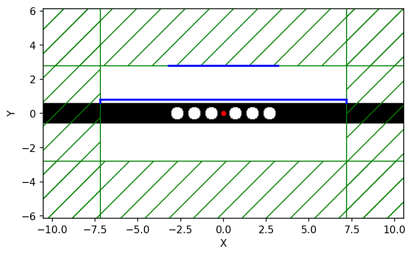
The simulation setup is shown in the schematic below. The binary grating has Λ = 1 μm at a wavelength of 0.5 μm via a normally-incident planewave pulse (which must extend into the PML region in order to span the entire width of the cell). The grating structure is terminated with a flat-surface padding in order to give the scattered field space to decay at the edge of the cell.

The simulation script is in examples/finite_grating.ctl.
;; true:  plot the scattered fields in the air region adjacent to the grating
;; false: plot the diffraction spectra based on a 1d cross section of the scattered fields
(define-param field-profile? true)

(set-param! resolution 50)                   ; pixels/μm

(define-param dpml 1.0)                      ; PML thickness
(define-param dsub 2.0)                      ; substrate thickness
(define-param dpad 1.0)                      ; flat-surface padding
(define-param dair                           ; air region thickness adjacent to grating
  (if field-profile? 10 dpad))
(define-param gp 1.0)                        ; grating periodicity
(define-param gh 0.5)                        ; grating height
(define-param gdc 0.5)                       ; grating duty cycle
(define-param num-cells 5)                   ; number of grating unit cells

(define-param wvl 0.5)                       ; center wavelength
(define fcen (/ wvl))                        ; center frequency

(set! k-point (vector3 0))

(define glass (make medium (index 1.5)))

(set! pml-layers (list (make pml (thickness dpml))))

(set! symmetries (list (make mirror-sym (direction Y))))

(define sx (+ dpml dsub gh dair dpml))
(define sy (+ dpml dpad (* num-cells gp) dpad dpml))

(set! geometry-lattice (make lattice (size sx sy no-size)))

(define src-pt (vector3 (+ (* -0.5 sx) dpml (* 0.5 dsub))))
(define pw-source (list (make source
                          (src (make gaussian-src (frequency fcen) (fwidth (* 0.2 fcen)) (is-integrated? true)))
                          (component Ez)
                          (center src-pt)
                          (size 0 sy))))
(set! sources pw-source)

(set! geometry (list (make block
                       (material glass)
                       (size (+ dpml dsub) infinity infinity)
                       (center (+ (* -0.5 sx) (* 0.5 (+ dpml dsub)))))))

(define mon-pt (vector3 (- (* 0.5 sx) dpml (* 0.5 dair))))
(define flat-fields (add-dft-fields (list Ez) fcen fcen 1 (volume (center mon-pt) (size (if field-profile? dair 0) (- sy (* 2 dpml))))))

(run-sources+ 100)

(output-dft flat-fields "flat")

(reset-meep)

(set! pml-layers (list (make pml (thickness dpml))))

(set! symmetries (list (make mirror-sym (direction Y))))

(set! geometry-lattice (make lattice (size sx sy no-size)))

(set! k-point (vector3 0))

(set! sources pw-source)

(set! geometry (list (make block
                       (material glass)
                       (size (+ dpml dsub) infinity infinity)
                       (center (+ (* -0.5 sx) (* 0.5 (+ dpml dsub)))))))

(set! geometry (append geometry
                       (map (lambda (n)
                              (make block
                                (material glass)
                                (size gh (* gdc gp) infinity)
                                (center (+ (* -0.5 sx) dpml dsub (* 0.5 gh)) (+ (* -0.5 sy) dpml dpad (* (+ n 0.5) gp)) 0)))
                            (arith-sequence 0 1 num-cells))))

(define grating-fields (add-dft-fields (list Ez) fcen fcen 1 (volume (center mon-pt) (size (if field-profile? dair 0) (- sy (* 2 dpml))))))

(run-sources+ 100)

(output-dft grating-fields "grating")
Results from the two HDF5 files are plotted using Matlab/Octave and shown for two finite gratings with 5 and 20 periods.
resolution = 50;
dpml = 1.0;
dsub = 2.0;
dpad = 1.0;
dair = 10;
gp = 1.0;
gh = 0.5;
num_cells = 5;
sx = dpml+dsub+gh+dair+dpml;
sy = dpml+dpad+num_cells*gp+dpad+dpml;

load "flat.h5";
flat_dft = ez_0_r+1j*ez_0_i;
load "grating.h5";
grating_dft = ez_0_r+1j*ez_0_i;
scattered_field = grating_dft-flat_dft;
scattered_amplitude = abs(scattered_field).^2;

field_profile = true;

if field_profile
   ### plot the scattered fields in the air region adjacent to the grating
   Nx = size(scattered_amplitude,2);
   Ny = size(scattered_amplitude,1);
   x = linspace(0.5*sx-dpml-dair,0.5*sx-dpml,Nx);
   y = linspace(-0.5*sy+dpml,0.5*sy-dpml,Ny);
   pcolor(x,y,scattered_amplitude);
   xlabel('x (um)');
   ylabel('y (um)');
   colormap("hot");
   shading interp;
   colorbar;
   caxis([0 max(max(scattered_amplitude))]);
   axis("equal","tight");
else
    ### plot diffraction spectra based on a 1d cross section of the scattered fields
    Ny = length(scattered_amplitude);
    y = linspace(-0.5*sy+dpml,0.5*sy-dpml,Ny);

    subplot(2,1,1);
    plot(y,scattered_amplitude,'bo-');
    xlabel("y (um)");
    ylabel("field amplitude");

    FT_scattered_amplitude = fftshift(fft(scattered_field));
    ky = [-Ny/2:(Ny/2-1)]*resolution/Ny;
    subplot(2,1,2);
    plot(ky,abs(FT_scattered_amplitude).^2,'ro-');
    axis([-3 3]);
    xlabel("wavevector k_y, 2π (um)^{-1}");
    ylabel("Fourier transform");
endif


The scattered field amplitude profile (the top figure in each of the two sets of results) shows that the fields decay to zero away from the grating (which is positioned at the left edge of the figure in the region indicated by the bright spots). The middle figure is the field amplitude along a 1d slice above the grating (marked by the dotted green line in the top figure). Note the decaying fields at the edges due to the flat-surface termination. The bottom figure is the Fourier transform of the fields from the 1d slice. As expected, there are only three diffraction orders present at ky=2πm/Λ for m=0, ±1, ±2. These peaks are becoming sharper as the number of grating periods increases.
The sharpness of the peaks directly corresponds to how collimated the diffracted beams are, and in the limit of infinitely many periods the resulting delta-function peaks correspond to diffracted planewaves. (The squared amplitude of each peak is proportional to the power in the corresponding diffraction order.) One can also obtain the collimation of the beams more directly by using Meep's near2far feature to compute the far-field diffracted waves — this approach is more straightforward, but potentially much more expensive than looking at the Fourier transform of the near field, because one may need a large number of far-field points to resolve the full diffracted beams. In general, there is a tradeoff in computational science between doing direct "numerical experiments" that are conceptually straightforward but often expensive, versus more indirect and tricky calculations that don't directly correspond to laboratory experiments but which can sometimes be vastly more efficient at extracting physical information.
In 3d, the procedure is very similar, but a little more effort is required to disentangle the two polarizations relative to the plane of incidence [the (z,k) plane for each Fourier component k]. For propagation in the direction, you would Fourier transform both and of the scattered field as a function of k . For each k, you decompose the corresponding E into the amplitude parallel to k [which gives the p polarization amplitude if you multiply by sec(θ), where sin(θ)=|k|/(nω/c), n is the refractive index of the ambient medium, and ω is the angular frequency; θ is the outgoing angle, where θ=0 is normal] and perpendicular to k [which equals the s polarization amplitude]. Then square these amplitudes to get something proportional to power as above. (Note that this analysis is the same even if the incident wave is at an oblique angle, although the k locations of the diffraction peaks will change.) Simulating large finite gratings is usually unnecessary since the accuracy improvements are negligible. For example, a 3d simulation of a finite grating with e.g. 100 periods by 100 periods which is computationally expensive would only provide a tiny correction of ~1% (on par with fabrication errors) compared to the infinite structure involving a single unit cell. A finite grating with a small number of periods (e.g., 5 or 10) exhibits weak diffractive effects and is therefore not considered a diffractive grating.
Far-Field Profile of a Cavity#
For this demonstration, we will compute the far-field spectra of a resonant cavity mode in a holey waveguide; a structure we had explored in Tutorial/Resonant Modes and Transmission in a Waveguide Cavity. The script is in examples/cavity-farfield.ctl. The structure is shown at the bottom of the left image below.
To set this up, we simply remove the last portion of examples/holey-wvg-cavity.ctl, beginning right after the line:
(set! symmetries
      (list (make mirror-sym (direction Y) (phase -1))
            (make mirror-sym (direction X) (phase -1))))
and insert the following lines:
(define-param d1 0.2)
(define nearfield
         (add-near2far fcen 0 1
           (make near2far-region (center 0 (+ (* 0.5 w) d1))
                                 (size (- sx (* 2 dpml)) 0))
           (make near2far-region (center (+ (* -0.5 sx) dpml) (+ (* 0.5 w) (* 0.5 d1)))
                                 (size 0 d1)
                                 (weight -1.0))
           (make near2far-region (center (- (* 0.5 sx) dpml) (+ (* 0.5 w) (* 0.5 d1)))
                                 (size 0 d1))))
We are creating a "near" bounding surface, consisting of three separate regions surrounding the cavity, that captures all outgoing waves in the top-half of the cell. Note that the x-normal surface on the left has a weight of -1 corresponding to the direction of the outward normal vector relative to the x direction so that the far-field spectra is correctly computed from the outgoing fields, similar to the flux and force features. The parameter d1 is the distance between the edge of the waveguide and the bounding surface, as shown in the schematic above, and we will demonstrate that changing this parameter does not change the far-field spectra which we compute at a single frequency corresponding to the cavity mode.
We then time step the fields until, at a random point, they have sufficiently decayed away as the cell is surrounded by PMLs, and output the far-field spectra over a rectangular area that lies outside of the cell:
(run-sources+ (stop-when-fields-decayed 50 Hz (vector3 0.12 -0.37) 1e-8))
(define-param d2 20)
(define-param h 4)
(output-farfields nearfield
 (string-append "spectra-" (number->string d1) "-" (number->string d2) "-" (number->string h))
 (volume (center 0 (+ (* 0.5 w) d2 (* 0.5 h))) (size (- sx (* 2 dpml)) h)) resolution)
The first item to note is that the far-field region is located outside of the cell, although in principle it can be located anywhere. The second is that the far-field spectra can be interpolated onto a spatial grid that has any given resolution but in this example we used the same resolution as the simulation. Note that the simulation itself used purely real fields but the output, given its analytical nature, contains complex fields. Finally, given that the far-field spectra is derived from the Fourier-transformed fields which includes an arbitrary constant factor, we should expect an overall scale and phase difference in the results obtained using the near-to-far-field feature with those from a corresponding simulation involving the full computational volume. The key point is that the results will be qualitatively but not quantitatively identical. The data will be written out to an HDF5 file having a filename prefix with the values of the three main parameters. This file will includes the far-field spectra for all six field components, including real and imaginary parts.
We run the above modified control file and in post-processing create an image of the real and imaginary parts of H over the far-field region which is shown in insets (a) above. For comparison, we compute the steady-state fields using a larger cell that contains within it the far-field region. This involves a continuous source and complex fields. Results are shown in figure (b) above. The difference in the relative phases among any two points within each of the two field spectra is zero, which can be confirmed numerically. Also, as would be expected, it can be shown that increasing d1 does not change the far-field spectra as long as the results are sufficiently converged. This indicates that discretization effects are irrelevant.
In general, it is tricky to interpret the overall scale and phase of the far fields, because it is related to the scaling of the Fourier transforms of the near fields. It is simplest to use the near2far feature in situations where the overall scaling is irrelevant, e.g. when you are computing a ratio of fields in two simulations, or a fraction of the far field in some region, etcetera.