Multilevel-Atomic Susceptibility#
This tutorial demonstrates Meep's ability to model saturable gain and absorption via multilevel atomic susceptibility. This is based on a generalization of the Maxwell-Bloch equations which involve the interaction of a quantized system having an arbitrary number of levels with the electromagnetic fields. The theory is described in Materials/Saturable Gain and Absorption. This example involves computing the lasing thresholds of a two-level, multimode cavity in 1d similar to the structure described in Figure 2 of Optics Express, Vol. 20, pp. 474-88, 2012.
First, the cavity consists of a high-index medium (\(n = 1.5\)) with a perfect-metallic mirror on one end and an abrupt termination in air on the other.
(set-param! resolution 400)
(define-param ncav 1.5)                          ; cavity refractive index
(define-param Lcav 1)                            ; cavity length
(define-param dpad 1)                            ; padding thickness
(define-param dpml 1)                            ; PML thickness
(define-param sz (+ Lcav dpad dpml))
(set! geometry-lattice (make lattice (size no-size no-size sz)))
(set! dimensions 1)
(set! pml-layers (list (make pml (thickness dpml) (side High))))
The properties of the polarization of the saturable gain are determined by the central transition's frequency ω\(_a\) and full-width half-maximum Γ as well as the coupling constant between the polarization and the electric field σ. Both ω\(_a\) and Γ are specified in units of 2π\(c\)/\(a\). As this example involves comparing results from Meep with the steady-state ab initio laser theory (SALT), we show explicitly how to convert between the different variable nomenclatures used in each method.
(define-param omega-a 40)                        ; omega_a in SALT
(define freq-21 (/ omega-a (* 2 pi)))            ; emission frequency  (units of 2πc/a)

(define-param gamma-perp 4)                      ; HWHM in angular frequency, SALT
(define gamma-21 (/ (* 2 gamma-perp) (* 2 pi)))  ; FWHM emission linewidth (units of 2πc/a)

(define-param theta 1)                           ; off-diagonal dipole matrix element
(define sigma-21 (* 2 theta theta omega-a))      ; dipole coupling strength (hbar = 1)
To understand the need for the high resolution, let us calculate the central wavelength of the lasing transition inside the high-index cavity relative to the cavity length:
The cavity contains roughly 10 wavelengths. This is an unphysically small cavity. Thus, to ensure that the electric field within the cavity is properly resolved, we have chosen roughly 40 pixels per wavelength, yielding a resolution of 400.
Next, we need to specify the non-radiative transition rates of the two-level atomic medium we're using as well as the total number of gain atoms in the system \(N_0\). The non-radiative transition rates are specified in units of \(c\)/\(a\).
(define-param rate-21 0.005)                     ; non-radiative rate  (units of c/a)
(define-param N0 37)                             ; initial population density of ground state
(define-param Rp 0.0051)                         ; pumping rate of ground to excited state
For a two-level atomic gain medium, the effective inversion that this choice of parameters corresponds to in SALT units can be calculated as:
The term in parenthesis on the right-hand side is the definition of \(D_0\) in normal units, and the additional factor of \(|\theta|^2 / \hbar \gamma_\perp\) converts to SALT's units.
(define two-level (make medium (index ncav)
        (E-susceptibilities (make multilevel-atom (sigma-diag 1 0 0)
          (transitions (make transition (from-level 1) (to-level 2) (pumping-rate Rp)
                             (frequency freq-21) (gamma gamma-21) (sigma sigma-21))
                       (make transition (from-level 2) (to-level 1) (transition-rate rate-21)))
          (initial-populations N0)))))

(set! geometry (list (make block (center 0 0 (+ (* -0.5 sz) (* 0.5 Lcav)))
                           (size infinity infinity Lcav) (material two-level))))
Definition of the two-level medium involves the multilevel-atom sub-class of the E-susceptibilities material type. Each radiative and non-radiative transition is specified separately. Note that internally, Meep treats pumping-rate and transition-rate identically, and you can use them interchangeably, but it is important to specify the from-level and to-level parameters correctly, otherwise the results will be undefined. The choice of these parameters requires some care. For example, choosing a pumping rate that lies far beyond the first lasing threshold will yield large inversion, and thus large gain, which is not realistic, as most physical devices will overheat before reaching such a regime. Meep will still produce accurate results in this regime though. Additionally, choosing the total simulation time is especially important when operating near the threshold of a lasing mode, as the fields contain relaxation oscillations and require sufficient time to reach steady state.
Also important is the definition of σ. When invoking the multilevel-atom sub-class of the E-susceptibilities material type, we need to specify the three components of sigma-diag, which is the direction pointed to by σ/|σ|. The magnitude |σ| is specified in the appropriate transition by sigma. Internally, Meep defines σ as (sigma sigma-21) * (sigma-diag 1 0 0). Thus, this saturable gain media will only couple to, and amplify, the E\(_x\) component of the electric field.
The field within the cavity is initialized to arbitrary non-zero values and a fictitious source is used to pump the cavity at a fixed rate. The fields are time stepped until reaching steady state. Near the end of the time stepping, we output the electric field outside of the cavity.
(init-fields)
(meep-fields-initialize-field fields Ex
             (lambda (p) (if (= (vector3-z p) (+ (* -0.5 sz) (* 0.5 Lcav))) 1 0)))

(define-param endt 7000)

(define print-field (lambda () (print "field:, " (meep-time) ", "
              (real-part (get-field-point Ex (vector3 0 0 (+ (* -0.5 sz) Lcav (* 0.5 dpad))))) "\n")))
(run-until endt (after-time (- endt 250) print-field))
The spectra of the field intensity is shown below.
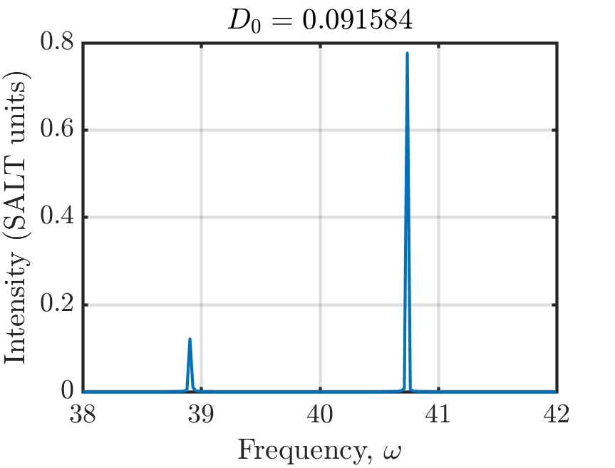
There are two lasing modes above threshold in the vicinity of the center transition frequency ω\(_a\)=40 as we would expect. Remember, when finding the frequency axis that Meep uses a Courant factor of \(\Delta t = 0.5 \Delta x\). We have also converted the electric field to SALT units using:
For two-level gain media, \(\gamma_\parallel = \gamma_{12} + \gamma_{21}\). We can also verify that the system is not exhibiting relaxation oscillations by directly plotting the electric field as a function of time and looking for very long time-scale oscillations. In the continuum limit, these modes would appear as Dirac delta functions in the spectra. The discretized model, however, produces peaks with finite width. Thus, we need to integrate a fixed number of points around each peak to calculate the correct modal intensity.
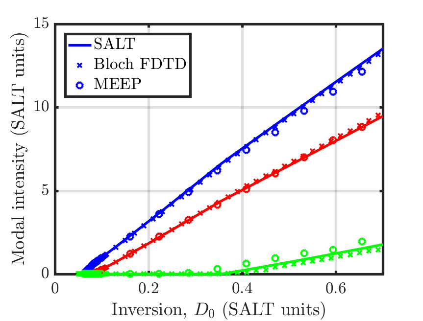
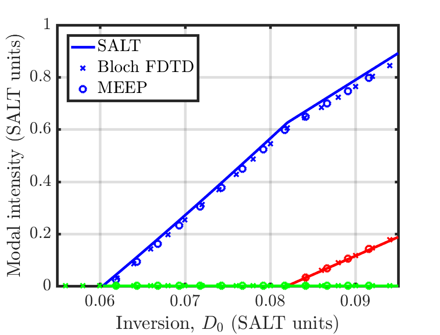
By varying \(N_0\) or the pumping rate \(R_p\), we can change the total gain available in the cavity. This is used to find the laser's modal intensities as a function of the strength of the gain. We can compare the simulated modal intensity with SALT as well as an independent FDTD solver based on the Maxwell-Bloch equations. All three methods produce results with good agreement close to the first lasing threshold.
Further increasing the gain continues to yield good agreement.